
News
Abbott Capital Management Celebrates 40 Years
Today, Abbott Capital Management marks its 40th anniversary, celebrating four decades of disciplined investing, enduring partnerships, and a longstanding commitment to serving its clients. S...


As the secondary market for private equity has grown substantially over the past few years, understanding the drivers behind secondary returns has become increasingly complex.
In this paper, we examine the risk-return profile of secondary transactions and discuss how diversification, discounts, and leverage all impact expected outcomes. We also review different reporting conventions and illustrate how reported performance metrics can differ significantly, depending on, for example, how recycled capital is accounted for.
There are five principal factors that determine the risk-return profile of a given secondary transaction and the corresponding MOIC1 and IRR2 metrics reported to investors:
1. Value appreciation of underlying assets
2. Diversification
3. Valuation and discounts
4. Transaction-level leverage
5. Recycling
Before reviewing each of these factors in detail, we look at the most common transaction types in the market today. Over the last several years, secondary buyers have started to target different transactions across the risk-return spectrum. In this context, the level of underlying asset diversification broadly determines the risk profile and corresponding target returns. Highly diversified, multi-fund portfolio transactions are typically underwritten to lower return targets (on an unlevered basis) when compared to concentrated single asset GP-led transactions. Such single asset transactions are often perceived as riskier and are therefore underwritten to higher returns. The following chart shows the four most common types of secondary transactions today.3
Chart 1: Secondary Transaction Types
Depending on the appetite for risk and the need for interim liquidity, an investor may be drawn towards either end of the diversification spectrum. That said, in addition to diversification, additional factors such as asset quality and corresponding value appreciation potential, valuation and discounts, transaction leverage, and recycling all impact the individual risk-return profile of a transaction.
In the following sections, we review these five factors and evaluate how each one impacts the expected outcome of secondary transactions.
We discuss practical questions such as:
In short, our aim is to “decode” the complexity of secondary returns by reviewing the underlying factors that drive returns and associated risks.
1. VALUE APPRECIATION OF UNDERLYING ASSETS
Fundamentally, private equity secondary transactions provide equity exposure to private companies. Therefore, one of the main return drivers is the value appreciation potential of the underlying portfolio companies. High-quality businesses that operate in attractive end markets generally have a higher potential to increase in value when compared to mediocre companies in lower growth markets. Investors in a secondary transaction should therefore focus their diligence on the quality of the underlying companies and the industries they operate in. A secondary investor diligencing a portfolio needs to address questions such as:
As part of the underwriting process, a secondary investor should understand and evaluate all relevant value drivers and associated risks of the underlying assets—because it is difficult to generate attractive secondary returns without value appreciation at the asset level.
While other factors can “shape” the risk-return profile of a secondary transaction, the evaluation of value appreciation potential and equity risk is at the core of every deal.
2. DIVERSIFICATION
Since Harry Markowitz introduced Modern Portfolio Theory in the early 1950s, investors have had a formal framework with which to manage the risk-return profile of diversified investment portfolios.5 Under this paradigm, idiosyncratic or unsystematic risks that are associated with a single stock or equity exposure can be reduced by holding a diversified basket of stocks whose returns are not perfectly positively correlated. For a secondary transaction, this means that more diversified transactions are generally perceived as less risky and are therefore typically underwritten to lower expected returns when compared to concentrated single asset transactions (see Chart 1). As such, a diversified secondary transaction is not inherently better or worse than a concentrated secondary transaction—it simply offers a different risk-return profile.
But is there such a thing as over-diversification? Warren Buffett’s position on this topic has been famously quoted as “wide diversification is only required when investors do not understand what they are doing.” Modern Portfolio Theory suggests that the marginal benefit of diversification decreases significantly for equity portfolios of more than 20-30 positions. A secondary transaction that provides exposure to hundreds of underlying companies may significantly reduce the element of unsystematic risk, but it is also unlikely that an investor will be able to generate meaningful outperformance. Put differently, it is difficult to beat an index if an investor’s portfolio substantially mirrors said index.
This also ties to Factor 1 discussed above, the value appreciation potential of the underlying assets. There is no point in identifying companies with value appreciation potential and diligencing individual equity risk if an investor then proceeds to invest in portfolios that contain almost every company included in the index universe.
3. VALUATION AND DISCOUNTS
As with any equity investment, the valuation at entry matters for the expected return outcome. For secondary transactions, there are two valuation levels that a buyer must consider:
i. the valuation at which the underlying GP is holding the assets as of a specific reference date, and;
ii. the price that the buyer is willing to pay to the seller as part of the transaction.
In a first step, a secondary investor must evaluate the GP’s valuation. Are the portfolio companies valued fairly? Is the GP applying conservative valuation multiples or are the companies marked aggressively?
Having formed a view on the GP’s valuations and having projected future proceeds from the portfolio, secondary buyers then focus their underwriting efforts on determining what price to offer the seller. That price, typically expressed as a percentage of the reference date NAV6, represents the “discount” or “premium” applied to a given transaction.
Secondary buyers often (but not always) bid at a discount relative to the reference date NAV. Via the discount, buyers can express their views on the underlying GP’s valuation and calibrate their investment according to the expected proceeds, their specific cost of capital and return targets. In this context, the discount to NAV “at the buy” provides the potential for an immediate unrealized gain because of the common industry practice that secondary buyers mark the position back up to the GP’s reported NAV after closing.
For example, if a buyer transacts at 90% of the NAV of a fund position, the buyer will be able to show an unrealized return of 1.11x MOIC as of the first day of ownership. A calendar quarter after closing the transaction, and all else being equal, the secondary buyer will report a 53.3% IRR. This represents the annualized IRR that corresponds to the 1.11x gross MOIC “achieved at the buy” in one quarter. However, with the passing of time, the reported IRR driven purely by the discount will decrease rapidly and will fall to just 7.3% after 1.5 years (six quarters) post close.
Chart 2: Reported Transaction Gross IRRs Over Time
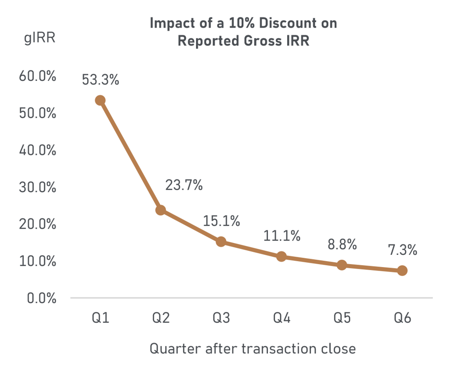
As shown in Chart 2, the discount can have a significant impact on the reported short-term unrealized performance of a secondary transaction. But how important are discounts for the ultimate long-term outcome of a transaction?
To better understand the impact, we compare two scenarios. In scenario one, a secondary buyer acquires an LP fund position with no discount (purchasing at 100% of NAV). We further assume that, over the course of the hold period, the fund assets appreciate and generate distributions to the secondary buyer of 60% more than the initial NAV at transaction close, resulting in a 1.60x MOIC attributable to value appreciation only. In scenario two, a secondary buyer acquires the same LP fund position at a 10% discount (purchasing at 90% of NAV). Assuming the same value appreciation of 1.60x, due to the initial discount, the same secondary transaction would generate a return of 1.78x MOIC. While the impact of the discount is meaningful for the overall return outcome, most of the return is still being generated by the appreciation of the underlying portfolio companies and not the discount.
Chart 3 shows the impact of discount levels between 0% (often called “par” pricing) and 10.0% on the return of a secondary transaction that otherwise generates a 1.60x MOIC and 16.9% IRR at par, i.e., through value appreciation only.7
Chart 3: Secondary Transaction Returns and Pricing Sensitivity
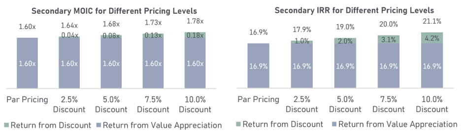
While discounts can enhance returns, the underlying value appreciation of the portfolio companies still typically represents the key performance driver.
4. TRANSACTION-LEVEL LEVERAGE
The use of transaction-level leverage to fund a secondary purchase has become increasingly common, especially for large and diversified multi-fund LP portfolio transactions.
For example, let’s assume that the buyer of a large, diversified $500m NAV LP portfolio might seek to borrow up to 30-40% LTV as transaction-level acquisition financing. This non-recourse financing would generally be backed solely by the portfolio of purchased LP positions. In addition, let’s assume that banks are pricing these loans at rates of SOFR + ~250-300bps (actual pricing would of course depend on the quality of the underlying funds). Assuming a SOFR level of 3.75%, annual cash interest payments would amount to ~6.25%-6.75%. For an LTV of 40%, the purchased portfolio would need to generate a minimum of ~2.5%-2.7% in annual distributions to service the cash interest payments due.
Given that distributions from a portfolio can be lumpy and are difficult to predict, amortization of such a loan could be based on an agreed upon cash sweep schedule. A bank and a secondary buyer may agree on a formula stipulating that, for example, 1.5x of the outstanding LTV is the cash sweep percentage used for the annual loan amortization. For a loan executed at 40% LTV, this means that in Year 1, 60% (1.5x*40%) of all portfolio distributions are used to pay down the principal portion of the loan. Following the amortization in Year 1 and a correspondingly lower LTV of, for example, 30% in Year 2, the second-year cash sweep would then be 45% (1.5x*30%), and so forth. Portfolio distributions not needed to amortize the loan (i.e., 40% in Year 1 and 55% in Year 2) can be used as distributions to equity investors in the secondary transaction.
While acquisition financing can enhance the equity return profile of a transaction, these benefits can erode quickly when portfolio distributions are lower than expected or delayed.
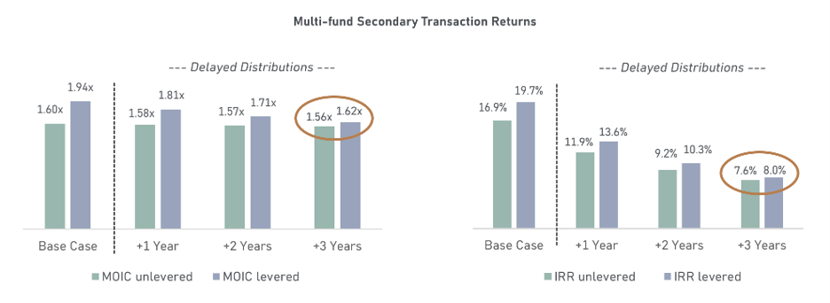
Below, we look at the impact of transaction-level leverage on the return expectations for a multi-fund LP portfolio purchase and review how a delay in distribution activity impacts levered and unlevered returns. The illustrative example is based on a $500m NAV LP portfolio that is purchased with 40% acquisition financing, requiring total annual interest payments of 6.5%.8 Due to leverage, the unlevered base case returns can be boosted from 1.60x and a 16.9% IRR to a 1.94x and a 19.7% IRR on a levered basis.9
As shown in Chart 4, leverage can meaningfully impact the base case return profile of a secondary transaction. However, since debt has costs and must be fully amortized before equity investors get to enjoy the full remaining upside, delays in distribution activity can quickly lower the benefits from leverage. In a muted distribution environment, the loan balance will be outstanding for longer (due to slower amortization via the sweep mechanism), which leads to higher absolute interest payments and correspondingly lower levered returns. As shown in Chart 4, an average delay of ~3 years in distributions relative to the base case can almost fully erode the initial benefits from leverage.
While the below analysis only looks at the timing of distributions, any shortfall in distribution amounts relative to the base case will also impact the return outcome. As with any type of leverage, if unlevered portfolio returns dip below the cost of borrowing, levered returns will fall below unlevered returns, and any potential losses would be exacerbated.
Chart 4: Return Impact from Leverage and Delay in Distributions
5. RECYCLING
The first four factors discussed so far all have a direct impact on the risk-return characteristics of a secondary transaction. It clearly matters how much value is created at the company level, how diversified a deal is, what discount a secondary investor can achieve “at the buy,” and how much transaction-level leverage is applied. However, when it comes to reported returns, it also matters how contributions and distributions are accounted for and how cash flow recycling is treated. Depending on the method applied, two investors in the same secondary transaction may report different return metrics.
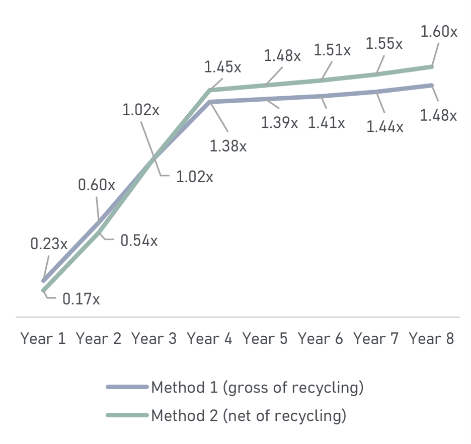
One of the key attributes of a secondary transaction is the potential for early liquidity. This is especially true for multi-fund and single-fund LP transactions but, to a lesser extent, also for certain multi-asset GP-led deals. Distributions received early in a transaction’s hold period can be used to offset future capital calls, resulting in a cash flow profile such as the one outlined in the example below. The example illustrates a hypothetical secondary multi-fund LP portfolio transaction with a purchase price of $100m at entry and unfunded commitments for future capital calls of $25m.
As outlined, distributions start as early as in Year 1 and are used to offset any future contributions, resulting in positive net cash flows in Years 1-8. In this context, there are two different reporting methods that calculate performance gross and net of recycling (i.e., cash flow offsets):
Chart 5: Secondary MOIC Gross and Net of Recycling
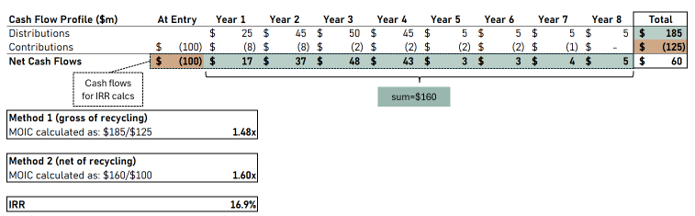
The IRR associated with the secondary transaction in the example is 16.9%. Given that the IRR formula considers one single “net” data point for a given cash flow date, one can argue that it is more closely linked to method 2, where cash flows are accounted for net of recycling.
How cash flow offsets are treated also impacts the reported DPI ratio. In the example below and following Method 1, the reported DPI metric at the end of Year 2 is 0.60x, calculated as $70m of distributions divided by $116m of contributions (i.e., paid-in capital). Under Method 2, the reported DPI in Year 2 is slightly lower at 0.54x, calculated as $54m of distributions divided by $100m of paid-in capital.
The chart below shows the difference in the reported DPI ratio for each method over time. Under the example, Method 1 shows slightly greater DPI in the earlier years of the transaction, whereas Method 2 ultimately leads to higher reported DPI numbers in the later years due to the cash flow offsets as DPI approaches the final MOIC outcome.
Chart 6: Recycling and DPI Progression
When analyzing the return profile of a secondary transaction, an investor should understand how recycling is treated for performance reporting. Different methodologies can lead to different metrics at different points in time, making it potentially difficult to compare reported performance metrics across transactions.
CONCLUDING THOUGHTS
Not all secondary returns are created equal. As the secondary market has matured, the range of transaction types has become increasingly broad. There is a substantial difference between, for example, (i) a single asset GP-led opportunity, and (ii) a large multi-fund LP portfolio that is purchased at a significant discount and levered at the transaction level.
Each of the five factors discussed in this paper impacts the risk-return profile of a given transaction. To truly understand secondary returns, an investor needs to evaluate how much each factor impacts the expected outcome of a transaction, a task that can be challenging but is not impossible. Breaking down the return drivers into value appreciation, discount, leverage, and recycling is a key step towards better understanding the increasingly broad and complex universe of secondary transactions.

1 Multiple of Invested Capital.
2 Internal Rate of Return.
3 We exclude NAV-based lending, preferred equity, and credit secondary transactions since they represent an altogether different risk-return category when compared to purely equity focused secondary transactions.
4 Target returns are hypothetical and aspirational in nature and are intended to provide information for the intended recipient only. Any hypothetical, composite or pro forma information contained herein is for illustrative purposes only and is not indicative of any future performance and does not reflect the actual or expected results achieved. There is no assurance the recipient will be able to achieve target results or make any profit or be able to avoid incurring substantial losses. Abbott has not applied any specific criteria when determining target performance and assumes favorable market conditions. Upon request, Abbott will provide additional information necessary to enable the recipient to understand the risks and limitations of using hypothetical performance in making investment decisions, including, without limitation, Abbott’s view of the likelihood of the target returns being achieved and any additional assumptions regarding the occurrence of future events. See Important Information Pages herein including Important Information about Target Hypothetical Returns.
Information included herein should not be relied upon when making investment decisions.
5 Markowitz, H.M. (March 1952), “Portfolio Selection”, The Journal of Finance.
6 Net Asset Value.
7 Assuming a 3-year average hold period.
8 The hypothetical model further assumes an additional 10% of future contributions to meet unfunded obligations at the portfolio level and a 9-year distribution pattern (85% of the portfolio is realized during the first 6 years of the hold period). The cash sweep percentage for debt amortization used in the example scales down from 60% in year 1 to 30% by year 5.
9 Unlevered and levered portfolio returns are calculated net of recycling.
10 Institutional Limited Partners Association.
IMPORTANT INFORMATION
This information is presented solely for informational purposes and should not be viewed as a current or past recommendation or an offer to sell or the solicitation to buy securities or adopt any investment strategy. Offerings are made only pursuant to a private offering memorandum containing important information. The opinions expressed herein represent the current, good faith views of the author(s) at the time of publication. There is no assurance that any events or projections will occur, and outcomes may be significantly different than the opinions shown here. This information, including any projections concerning financial market performance, is based on current market conditions, which will fluctuate and may be superseded by subsequent market events or for other reasons.
Unless otherwise noted, all charts and figures in this paper are hypothetical, simplified, and intended solely to illustrate general concepts discussed herein. They do not represent the actual or projected performance of any fund, account, or investment managed by Abbott, and should not be relied upon in making any investment decision. Hypothetical performance has inherent limitations; it does not reflect actual trading, liquidity constraints, fees, or market conditions, and actual results may differ materially.
Past performance is not a guide to future results and is not indicative of expected realized returns.
Copyright© Abbott Capital Management, LLC 2026. All rights reserved. This material is proprietary and may not be reproduced or distributed without Abbott’s prior written permission. It is delivered on an “as is” basis without warranty or liability. Abbott accepts no responsibility for any errors, mistakes or omissions or for any action taken in reliance thereon. All charts, graphs and other elements contained within are also copyrighted works and may be owned by Abbott or a party other than Abbott.
The views and information provided are as of July 2026 unless otherwise indicated and are subject to frequent change, update, revision, verification and amendment, materially or otherwise, without notice, as market or other conditions change. There can be no assurance that terms and trends described herein will continue or that forecasts are accurate. Certain statements contained herein are statements of future expectations or forward-looking statements that are based on Abbott’s views and assumptions as of the date hereof and involve known and unknown risks and uncertainties (including those discussed below and in Abbott’s Form ADV Part 2A, available on the SEC’s website at www.adviserinfo.sec.gov) that could cause actual results, performance or events to differ materially and adversely from what has been expressed or implied in such statements. Forward-looking statements may be identified by context or words such as “may, will, should, expects, plans, intends, anticipates, believes, estimates, predicts, potential or continue” and other similar expressions. Neither Abbott, its affiliates, nor any of Abbott’s or its affiliates’ respective advisers, members, directors, officers, partners, agents, representatives or employees or any other person is under any obligation to update or keep current the information contained in this document.
This material is for informational purposes only and is not an offer or a solicitation to subscribe to any fund and does not constitute investment, legal, regulatory, business, tax, financial, accounting or other advice or a recommendation regarding any securities of Abbott, of any fund or vehicle managed by Abbott, or of any other issuer of securities. No representation or warranty, express or implied, is given as to the accuracy, fairness, correctness or completeness of third-party sourced data or opinions contained herein and no liability (in negligence or otherwise) is accepted by Abbott for any loss howsoever arising, directly or indirectly, from any use of this document or its contents, or otherwise arising in connection with the provision of such third-party data.
Today, Abbott Capital Management marks its 40th anniversary, celebrating four decades of disciplined investing, enduring partnerships, and a longstanding commitment to serving its clients. S...

We are pleased to share our Q1 2026 Private Equity Market Overview.

Private equity investing has long thrived on a few key principles: a focus on the long-term, the ability to remain patient, and the maintenance of a steady and consistent commitment pace to ...